Quantopian zipline trading algorithm parameter optimization with Spearmint Bayesian Optimizer - Part 1
Quantopian’s zipline - a Pythonic Algorithmic Trading Library – is a powerful platform for creating automated trading algorithms. Algorithms almost always have tuning parameters that control the entry or exit rules for trades.
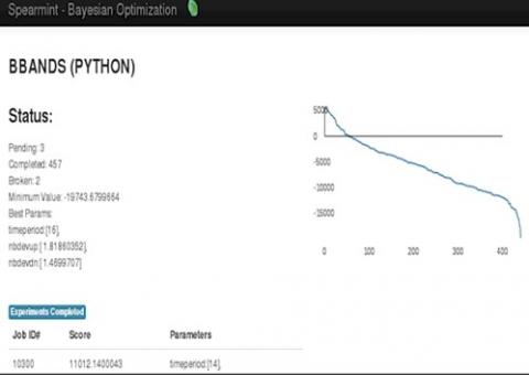
As an example, a trading algorithm using Bollinger Bands (referred to as BBANDS) has three free parameters. The first is an integer time period for the look-back. The other two are floating point numbers for the “up” and “down” deviation for the trading signal. To optimize such an algorithm using a grid scan to explore all combinations is an immense task.
Currently, neither Quantopian nor zipline offer a built in method of optimizing tuning parameters.
Quantopian’s blog entry on this problem listed a few alternatives, one of which is the Spearmint Bayesian Optimizer open source tool kit. The results to me were very impressive.
I selected a Bollinger Band algorithm to trade the SPY ETF for 2014 because - as experienced quants already know – my chances of successfully curve fitting it against one equity and one years worth of data are very high. And to state the obvious, the algo tuned optimally for SPY in 2014 would not do as well in other years or for other stocks or periods. This means that this algo is just a platform for exploring how to economically best fit tuning parameters using a Bayesian optimizer and not to design a practical money maker.
Figure 1 is the quantopian version of the algo, and can be downloaded here . (Or, download all files used here ).
|
1 2 3 4 5 6 7 8 9 10 11 12 13 14 15 16 17 18 19 20 21 22 23 24 25 26 27 28 |
import talib def initialize(context): context.secs = [ symbol('SPY') ] context.history_depth = 30 context.iwarmup = 0 context.BBANDS_timeperiod = 16 context.BBANDS_nbdevup = 1.819 context.BBANDS_nbdevdn = 0.470 def handle_data(context, data): context.iwarmup = context.iwarmup + 1 if context.iwarmup <= ( context.history_depth + 1 ) : return dfHistD = history(30, '1d', 'price') S=context.secs[0] CurP=data[S].price BolU,BolM,BolL = talib.BBANDS( dfHistD[S].values, timeperiod=context.BBANDS_timeperiod, nbdevup=context.BBANDS_nbdevup, nbdevdn=context.BBANDS_nbdevdn, matype=0) record(CurP=CurP,BolU=BolU[-1],BolM=BolM[-1],BolL=BolL[-1]) if CurP < BolL[-1] : order_target_percent(S,+0.97) else: if CurP > BolU[-1] : order_target_percent(S,-0.97) return |
|
|
Figure 1 : Quantopian version of the BBANDS Trading Algorithm |
Lines 4 to 5, and 10 to 12, for warming the history dataframe are not needed on Quantopian, but are included so that we can compare the results with the zipline version.
Lines 23 to 27 contain the minimal trading logic, which is to sell when the current price drops below the lower Bollinger line and buy when it exceeds the uppder. The algo can go both long and short to 97% of its portfolio value.
You can see the three algo tuning parameters are defined in lines 6 thru 9, and are passed to the ta-LIB BBAND function in lines 18 to 20. So, any quant who is looking for evidence of curve-fitting will ask where did the tuning constants in lines 6-9 come from?
Read Part 2 for how they were determined.